The question
Transformer bottlenecks are widely reported to improve medical segmentation. But a paper that introduces a Transformer usually also introduces a pretraining scheme, a new augmentation policy and a longer schedule — and reports the combined gain. That leaves the actual source of the improvement unattributed.
This project holds everything else fixed and varies two things independently: the architecture (CNN U-Net vs. TransUNet) and the initialisation (random vs. SimCLR-pretrained). Three configurations are enough to separate them.
Results
| Model | Validation DSC | Public test DSC | Generalisation gap |
|---|---|---|---|
| Simple CNN U-Net | 0.71459 | 0.6983 | 0.01629 |
| TransUNet (randomly initialised) | 0.71499 | 0.5136 | 0.20139 |
| TransUNet + SimCLR pretraining | 0.73544 | 0.7316 | 0.00384 |
Adding a Transformer bottleneck changed validation Dice by 0.0004. Not a small improvement — nothing at all, well inside run-to-run noise. On its own, the architecture bought no performance.
Pretraining the same architecture with SimCLR raised it by 2.9% on validation and 3.3% on the public test set, and cut the validation-to-test generalisation gap from 0.016 to 0.004 — a factor of four against the CNN baseline.
The conclusion the experiment supports is narrow and worth stating precisely: on this dataset, the Transformer bottleneck is not what helps. What helps is initialising its encoder with features learned from the unlabelled images. Architecture without the right initialisation was inert.
A caveat about the second row, stated because it weakens my own result. The TransUNet-without-SSL public score of 0.5136 was produced while the configuration still contained an architecture error from early experimentation, and was not re-run after that was fixed. That number is not a fair comparison, and the apparent 21.8% gain over it should be discounted entirely. The defensible comparison — and the one the claim above rests on — is against the CNN U-Net baseline.
No external pretrained weights are used anywhere in this project. The ResNet50 encoder is always
instantiated with weights=None; the only pretraining is the SimCLR stage, performed on unlabelled
images from the same dataset. This is a hard constraint rather than a stylistic choice, and it is
also what makes the result interesting: the 2.9% comes from data that was already in hand, unlabelled.
Data
Grayscale medical images in TIFF format with binary masks, split 80/20 into training and validation with a fixed seed. Preprocessing resizes images bilinearly and labels with nearest-neighbour interpolation — using bilinear on a binary mask would silently produce fractional labels at every boundary, which is precisely where segmentation accuracy is decided.
Input resolutions differ by configuration: 256×256 for the CNN U-Net, 384×512 for TransUNet, and 448×576 for SimCLR pretraining.
Architectures
Simple CNN U-Net. Standard encoder–decoder with skip connections, channels progressing
1 → 64 → 128 → 256 → 512 → 1024 and back, DoubleConv blocks (two 3×3 convolutions with BatchNorm
and ReLU), transposed convolutions for learnable upsampling, and a 1×1 convolution to a single
output channel.
TransUNet. A ResNet50 encoder taken up to layer3 (1024 channels at 1/16 resolution), a ViT
bottleneck, and a U-Net-style decoder that reuses the ResNet’s intermediate features as skip
connections. The ViT has embedding dimension 384, depth 8, 6 heads, MLP ratio 3 and dropout 0.1.
Self-attention at 1/16 resolution supplies global context; the skip connections supply the
fine-grained spatial detail attention at that resolution cannot.
TransUNet + SimCLR. Architecturally identical. Only the ResNet encoder layers (conv1, bn1,
layer1, layer2, layer3) are transferred from the pretrained checkpoint; the ViT and the
decoder start random. The difference between rows two and three of the results table is exactly this
one substitution.
SimCLR pretraining
Contrastive learning on the unlabelled training images: two augmented views of the same image are pulled together in projection space while views of different images are pushed apart, under the NT-Xent loss
The projection head is a two-layer MLP (768 → 768 → 128) with L2 normalisation, discarded after pretraining.
The augmentation policy carries the whole method — it defines what the encoder is asked to treat as irrelevant. Random resized crop (scale 0.08–1.0), horizontal and vertical flips, ±15° rotation, mild affine jitter, Gaussian blur and Gaussian noise. Vertical flips are included here and absent from the supervised policy, which is deliberate: medical images of this kind have no canonical up, so orientation is genuinely nuisance information, and telling the encoder so is free supervision.
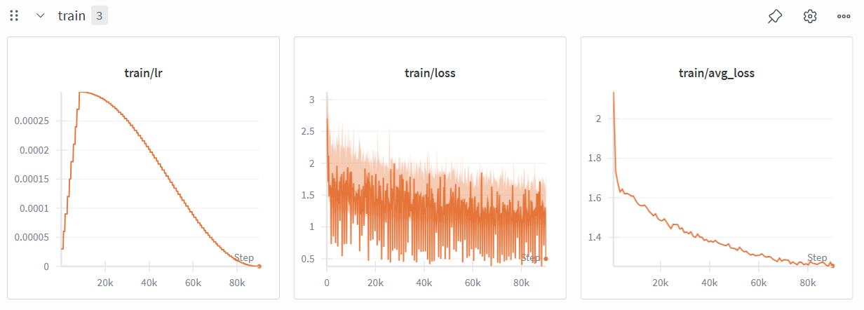
Trained 100 epochs, batch size 8, AdamW at lr 3e-4, with a 10-epoch linear warmup followed by cosine decay.
Training configuration
| CNN U-Net | TransUNet | TransUNet + SimCLR | |
|---|---|---|---|
| Epochs | 100 | 150 | 150 |
| Batch size | 4 | 8 | 8 |
| Optimiser | Adam | AdamW | AdamW |
| Learning rate | 1e-4 | 1e-4 | 1e-4 |
| Scheduler | CosineAnnealingLR | — | 5-epoch warmup, then adaptive |
| Input size | 256×256 | 384×512 | 384×512 |
Loss is a combined BCE + Dice objective, weighted equally with a smoothing factor of 1e-5. The two terms answer different questions — BCE scores every pixel independently, Dice scores the region overlap — and on a task where the foreground is a small fraction of the image, BCE alone is happy with a model that predicts almost nothing.
Model selection is on best validation Dice throughout.
Learning curves
| CNN U-Net | TransUNet | TransUNet + SimCLR | |
|---|---|---|---|
| Loss & learning rate | 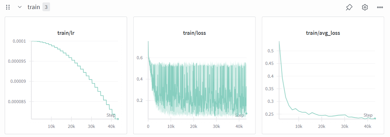 | 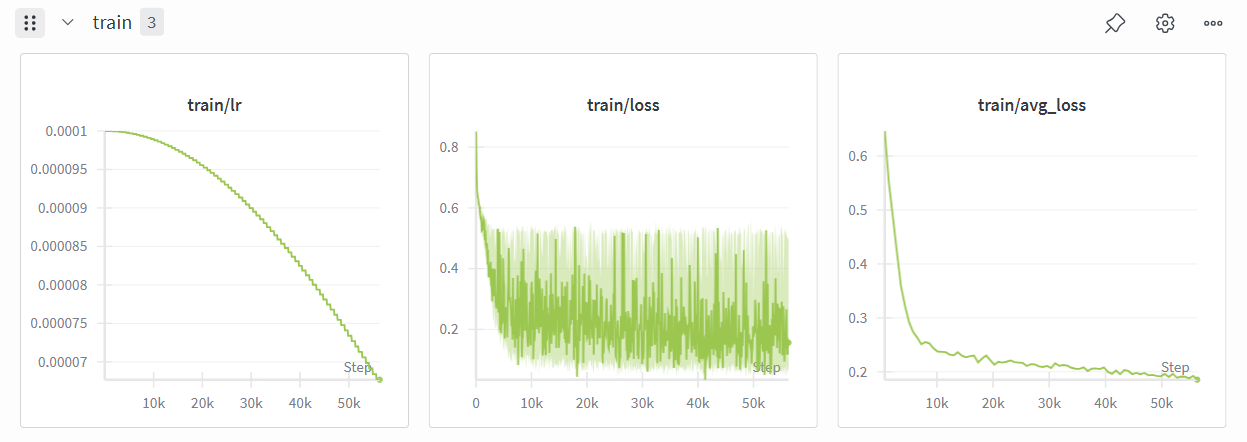 | 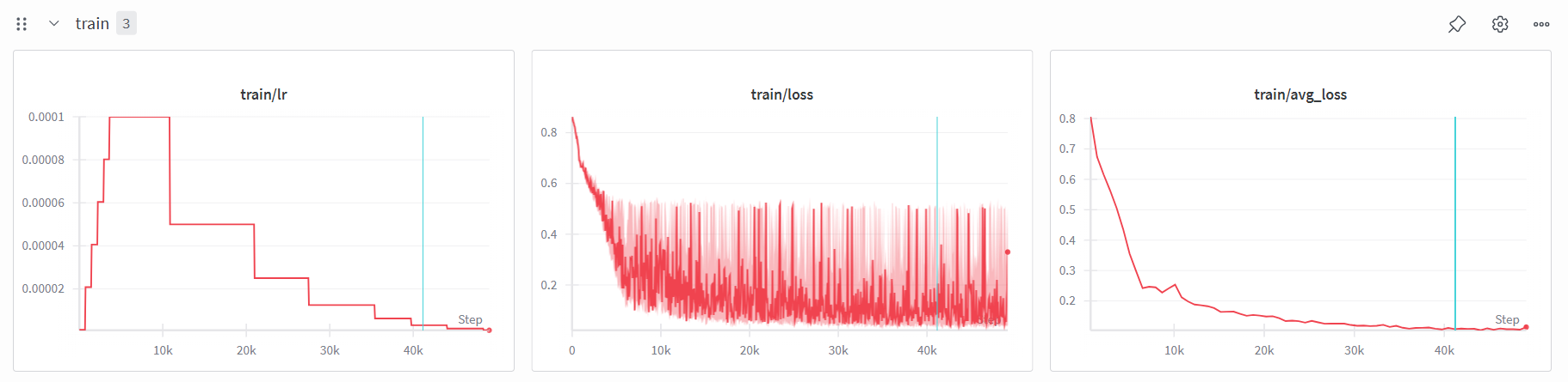 |
| Validation Dice | 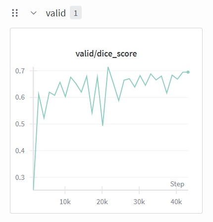 | 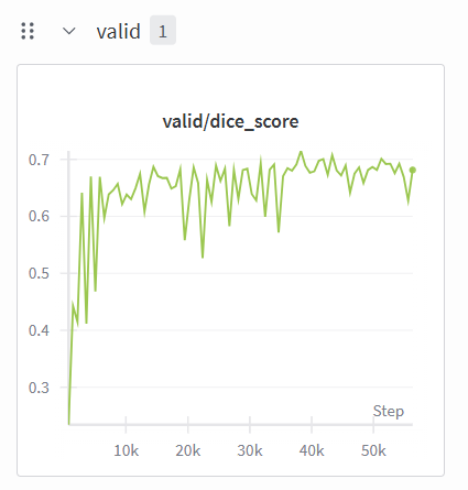 | 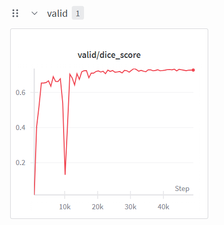 |
The curves show the effect that the final scores only imply. The randomly-initialised TransUNet fluctuates noticeably during training — a Transformer bottleneck at 1/16 resolution being asked to learn attention patterns from scratch on a small labelled set. With the SimCLR encoder in place the same architecture converges faster and more smoothly, and its validation performance is stable rather than jumpy.
That stability, not the headline 2.9%, is the most convincing evidence that the pretrained features are doing real work: better initialisation shows up as a better-conditioned optimisation problem, not just a better endpoint.