2D Generative Models — DDPM, DDIM, GAN, MeanFlow

The question

Generative models are usually compared on how good their samples look. On a 2D synthetic distribution that judgement can be replaced with a number: the target density is known exactly, so the distance between the generated and target distributions is directly measurable.

That makes it possible to ask a sharper question than “which model is best?” — namely, what does each sample actually cost? A GAN produces a sample with one forward pass. DDPM needs a thousand. If the thousand passes buy nothing, they are not worth paying for; if they do, the interesting question is how few of them are enough.

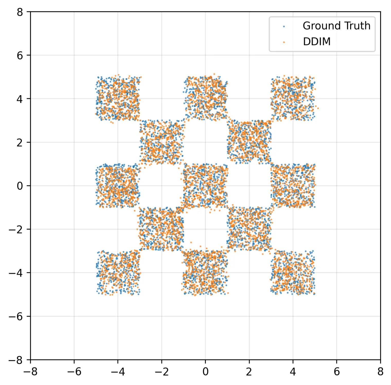
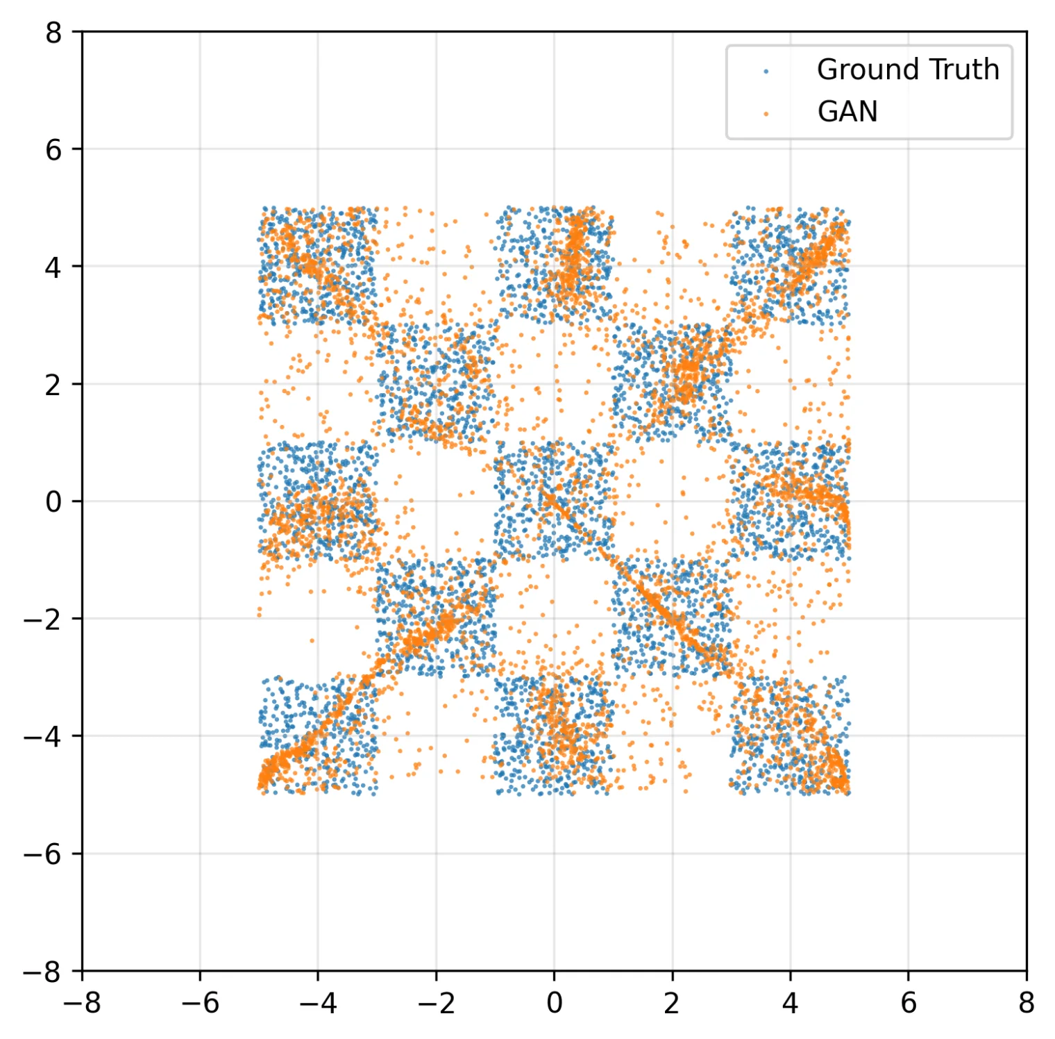
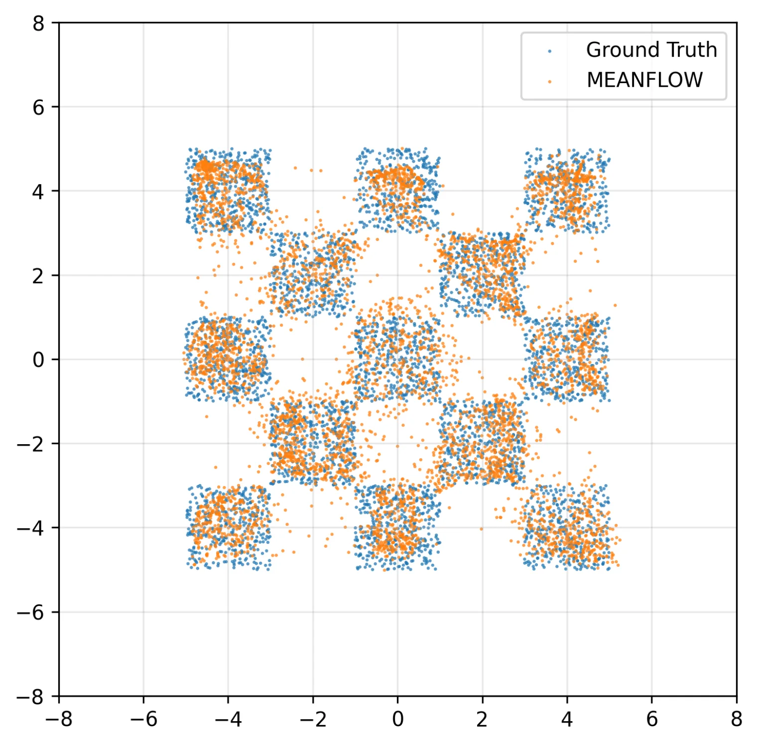
All four model families — GAN, DDPM, DDIM and MeanFlow — are implemented from scratch in PyTorch and trained on the checkerboard distribution, a deliberately awkward target: multi-modal, with sharp axis-aligned boundaries and large empty regions that a model can easily smear across.

Metrics

Two distances are reported, both computed against samples from the true distribution:

Energy distance (ED) — a kernel-free statistical distance, cheap and stable to estimate.
2-Wasserstein distance (WD) — the optimal-transport cost of moving one distribution onto the other,

W_2(\mu, \nu) = \left( \inf_{\gamma \in \Gamma(\mu,\nu)} \int \lVert x - y \rVert^2 \, d\gamma(x,y) \right)^{1/2}

where $\Gamma(\mu,\nu)$ is the set of couplings with marginals $\mu$ and $\nu$ . Unlike a likelihood, $W_2$ stays finite and informative when the two distributions have disjoint support — exactly the regime a partially-trained generator is in.

Reporting both matters: they disagree in places, and where they disagree is where the interesting behaviour is.

Results

DDIM is not a separately trained model: it loads the same checkpoint as DDPM and changes only the sampler, so the rows below differ in inference procedure alone. All DDIM rows use $\eta = 1.0$ .

Method	Steps (NFE)	ED	WD
GAN	1	0.0127	0.4700
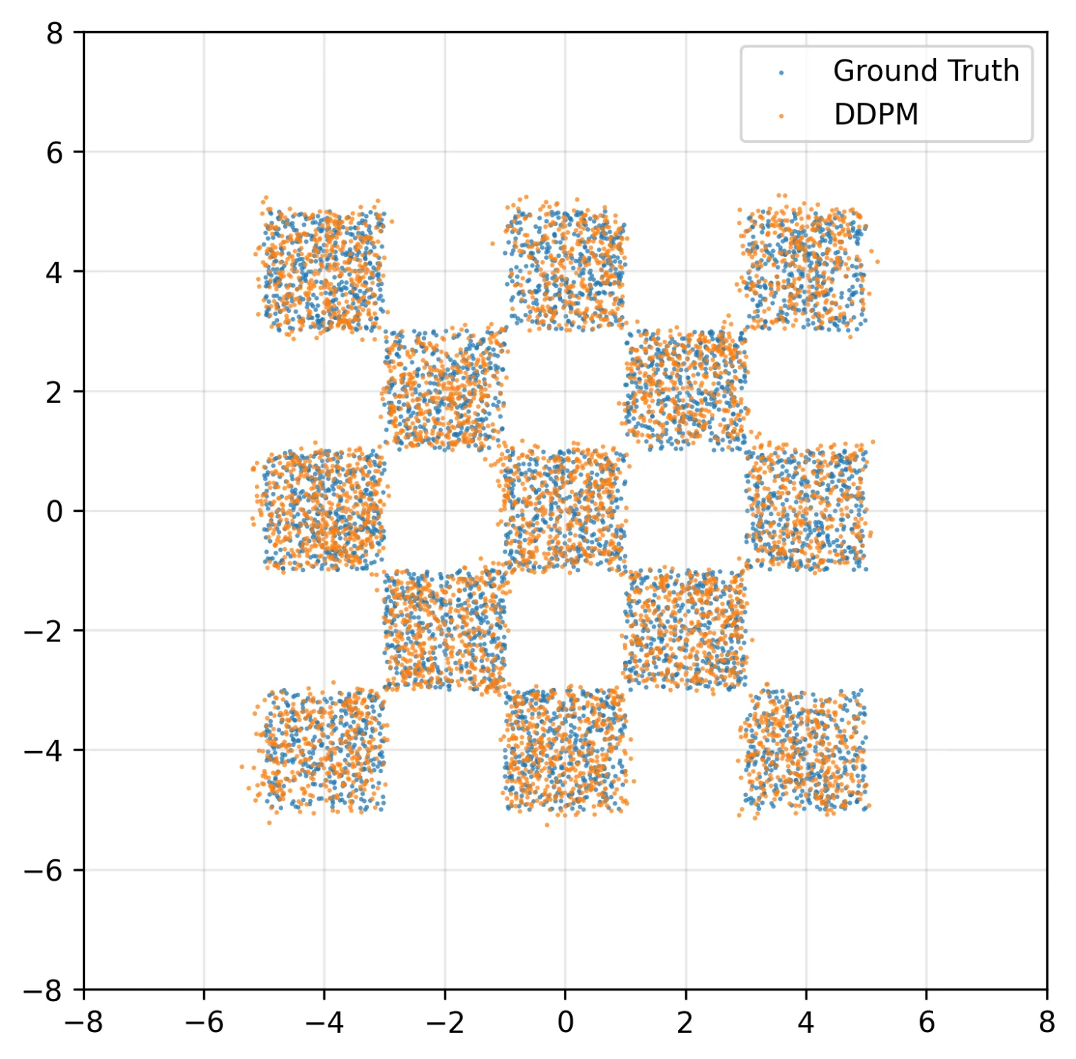
DDPM	1000	0.0025	0.2941
DDIM	1000	0.0025	0.2940
DDIM	500	0.0017	0.2106
DDIM	100	0.0013	0.2129
DDIM	10	0.0596	0.8685
DDIM	1	1.2627	4.0667
MeanFlow	1	0.0037	0.3464

Three things fall out of this table.

Most of the thousand steps are wasted. DDIM at 100 steps is not merely as good as DDPM at 1000 — it is better, on both metrics. A 10× reduction in sampling cost that improves quality is not a trade-off at all; the extra steps were adding noise, not signal.

The cliff is between 100 and 10 steps. At 10 steps ED jumps to 0.0596; at a single step the model produces essentially nothing usable (ED 1.2627). Whatever DDIM is doing, it cannot be compressed below roughly two orders of magnitude of steps.

One step is achievable, but not by shortening a diffusion trajectory. MeanFlow reaches ED 0.0037 in a single network evaluation — three times better than the GAN and a factor of 340 better than 1-step DDIM. Getting to 1-NFE generation required changing the training objective, not truncating the sampler.

DDPM, 1000 steps — the reference sample quality the others are measured against.

DDIM, 1000 steps — visually indistinguishable from DDPM, and numerically identical to four decimal places.

GAN, 1 step — the checkerboard structure is there, but points scatter across the boundaries that should be empty.

MeanFlow, 1 step — the same single-evaluation budget as the GAN, with boundaries close to DDPM's.

Ablation: how much stochasticity does DDIM want?

DDIM interpolates between a deterministic sampler and DDPM through the parameter $\eta$ : at $\eta = 0$ sampling is fully deterministic, at $\eta = 1$ it recovers DDPM’s stochastic update. Fixing the budget at 50 steps:

$\eta$	ED	WD
0	0.0112	0.4737
0.25	0.0067	0.3559
0.5	0.0068	0.3559
0.75	0.0045	0.3733
1.0	0.0046	0.3226

Deterministic sampling is the worst setting by a wide margin — more than double the ED of the best. The plausible reading is mode collapse: with no injected noise, every trajectory from a given starting point lands in the same place, and a checkerboard’s separated modes are exactly what that under-covers.

Ablation: time embedding

Time embedding	ED	WD
Learned	0.0052	0.2980
Sinusoidal	0.0025	0.2941

Fixed sinusoidal positional embedding halves the energy distance relative to a learned embedding. The denoiser is conditioned on a scalar timestep and needs a smooth, well-separated representation of it; the sinusoidal basis supplies that by construction, whereas a learned table has to discover it from a training signal that is only indirectly about time.

Training behaviour

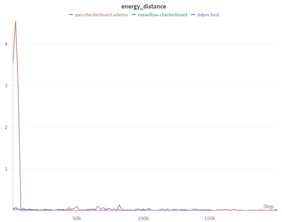
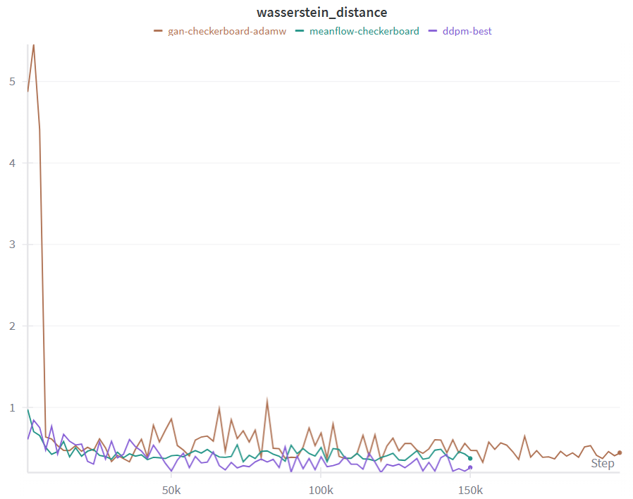
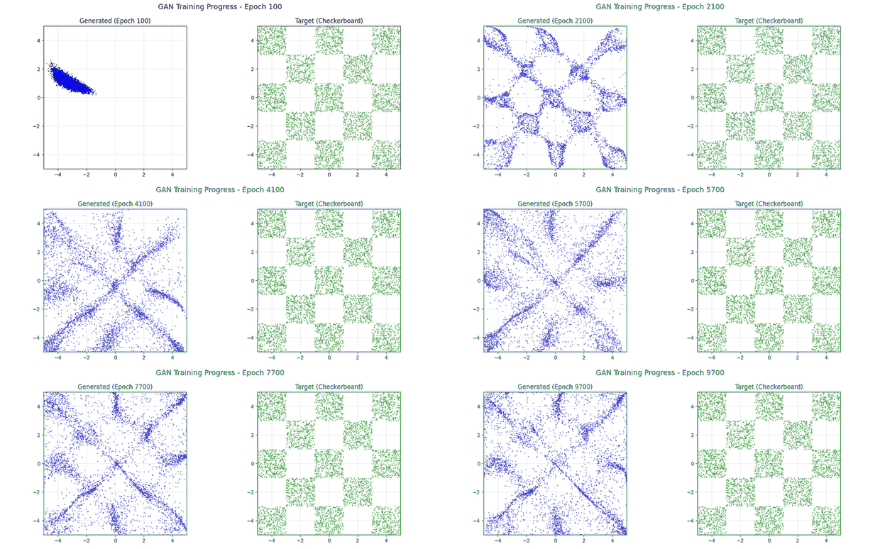
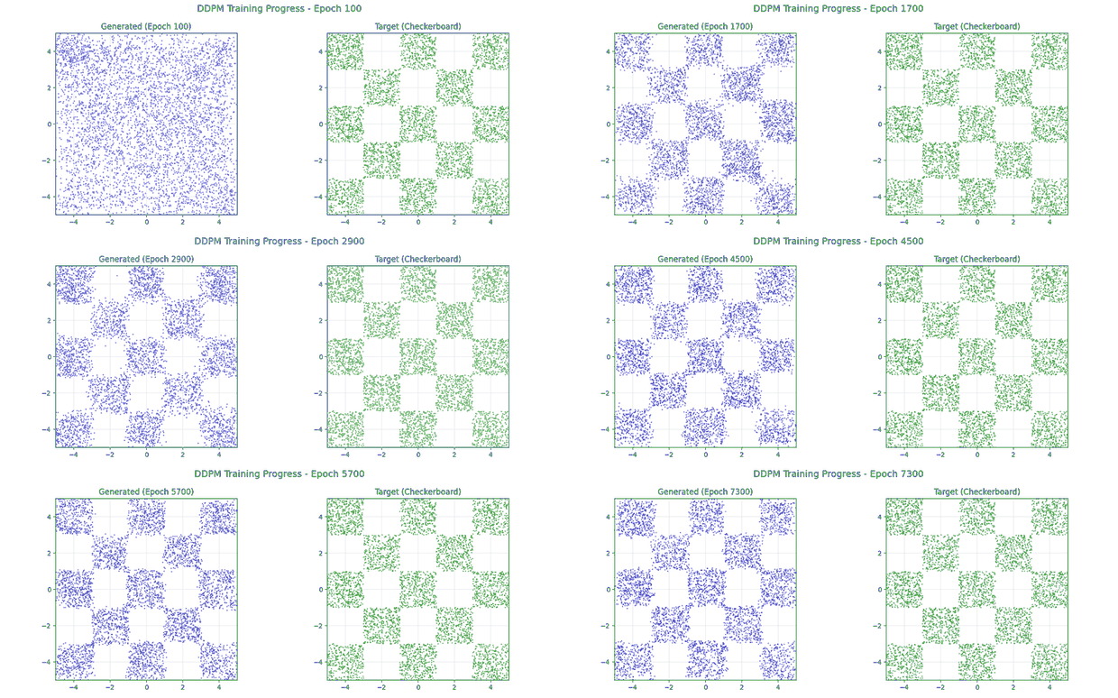
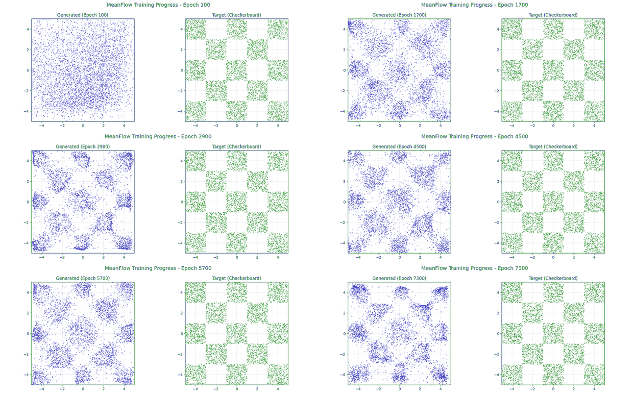
Energy distance against training epochs. DDPM and MeanFlow drop faster and settle lower than the GAN.

2-Wasserstein distance against training epochs. The same ordering holds under a second, unrelated metric.

The curves show the expected split in training character. GAN generator and discriminator losses oscillate against each other throughout, and the distribution metrics oscillate with them. DDPM’s noise-prediction MSE descends smoothly and flattens — the objective is a plain regression and behaves like one. MeanFlow, trained with a Huber loss and JVP-based targets, converges about as stably as DDPM despite generating in one step.

The animations show what a scalar metric cannot: which parts of the distribution are being won and lost while that number moves.

GAN — the global structure appears early, then modes wobble as generator and discriminator trade off.

DDPM — noise resolves into the checkerboard monotonically, with boundaries sharpening throughout.

MeanFlow — comparable convergence to DDPM, reached with a one-step sampler.